Cell Formatting
Number Tab
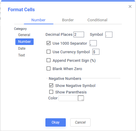
If a cell has a numeric, date, or time value use Number formatting to choose how the value should appear on the report. For example, add a dollar sign ($) to monetary values and separate each three digits to make values easier to read.
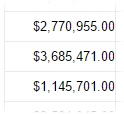
Numeric values with currency styled formatting
The following options for Number formatting are available:
General
This is the default option. The application will examine the data then set formatting automatically. There are a few rules to consider when choosing General based on what data type appears in the cell:
- The application will first check to see if the value is a number, then a date and then assume it is text if no other criteria are met.
- If the cell is determined to be a numeric value, and the Apply Numeric Decimal Places to General Cell Formatting feature is enabled by the system administrator, then a decimal separator character and a number of decimal places are included with the value. The number of places and the separator character are determined by the system configuration. To override these settings, change formatting to Number and set the corresponding settings.
- If the cell is determined to be a currency value, and the Apply General Currency Right Alignment feature is enabled by the system administrator, the value is automatically right-aligned in the cell.
Number
Format the data as a number, currency, or percentage. A number of optional settings control specific formatting options:
Tip
Leave the Symbol field, the Use 1000 Separator symbol field and Use Currency Symbol symbol field at their defaults when possible. This way, they can be automatically overridden by the application when the cultural or locale settings are changed. For example, the system can display
£in place of$. Setting a value for these symbols at the cell level will set that symbol for all executions of the report, regardless of cultural/locale settings.
- In the Decimal Places field, enter a number for how many decimal places to display.
- Use the Symbol field to override the system’s default decimal separator character. Changing the value of this field from the default will override the symbol for all executions of the report, regardless of the user’s local/culture settings. Leave as the default (or change back to the default) to allow the application to change the symbol based on local/culture settings.
- To show a delimiter every three digits, check the Use 1000 Separator checkbox. Then, in the field to the right, enter a symbol to use as the delimiter. Like the Symbol field, changing the value of this field from the default will override the symbol for all executions of the report, regardless of the user’s local/culture settings. Leave as the default (or change back to the default) to allow the application to change the symbol based on local/culture settings.
- To show a currency symbol before the number, check the Use Currency Symbol. Then, in the field to the right, enter the symbol to show. Like the Symbol field, changing the value of this field from the default will override the symbol for all executions of the report, regardless of the user’s local/culture settings. Leave as the default (or change back to the default) to allow the application to change the symbol based on local/culture settings.
- To show a percent sign (%) after the number, check the Append Percent Sign (%) checkbox.
- To show no value if the number is 0, check the Blank When Zero checkbox.
- To show a negative sign (-) in front of negative numbers, check the Show Negative Symbol checkbox.
- To show parentheses ( ) around negative numbers, check the Show Parenthesis checkbox.
- To show negative numbers in a different color, enter a hexadecimal color code in the Color field or use the color picker to choose a color.
Date
Format the data as a date, time, or date and time.
Optional: Choose which date and time components to display, and how to show them. Either:
- select one of the patterns from the Date/Time Format list, or
- enter a custom pattern using the following variables:
| Variable | Description | Result for sample date of “Sept-2-1907 5:08:04 PM” |
|---|---|---|
| d | day of the month, from 1 to 31 | 2 |
| dd | day of the month, from 01 to 31 | 02 |
| ddd | day of the week, abbreviated name | Mon |
| dddd | day of the week, full name | Monday |
| M | month, from 1 to 12 | 9 |
| MM | month, from 01 to 12 | 09 |
| MMM | month, abbreviated name | Sept |
| MMMM | month, full name | September |
| y | year of the century, from 0 to 99 | 7 |
| yy | year of the century, from 00 to 99 | 07 |
| yyyy | year, from 0001 to 9999 | 1907 |
| h | hour using a 12 hour clock, from 1 to 12 | 5 |
| hh | hour using a 12 hour clock, from 01 to 12 | 05 |
| H | hour using a 24 hour clock, from 0 to 23 | 17 |
| HH | hour using a 24 hour clock, from 00 to 23 | 17 |
| m | minute, from 0 to 59 | 8 |
| mm | minute, from 00 to 59 | 08 |
| s | second, from 0 to 59 | 4 |
| ss | second, from 00 to 59 | 04 |
| t | A/P | P |
| tt | AM/PM | PM |
Text
Does not apply any formatting to the data, and show it exactly as it appears in the data object.
Border
Alter the width and color of the cell borders. To set a color for a cell border, enter a color code or select a color from the picker. To set the width of the border, enter a pixel value, or use the arrows to make the border thicker or thinner.
To set all the cell borders to the same color and width, check the Make Borders Uniform checkbox.
Tip
If gridlines are enabled for the Report Viewer, then cell borders will show in addition to the gridlines.
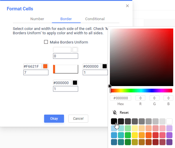
Choosing border colors and widths
Conditional Formatting
A conditional format allows you to format a cell according to its output data. The cell and text styles can depend on its data value, and you can even conditionally hide rows or entire sections. This can be useful for highlighting certain values in a data set, such as outliers from a trend.
Conditional Formatting uses a formula to set the condition. The formula must evaluate to True or False. If True, the formatting will be applied otherwise it will not. Conditional formulas are often based on data in the cell, but they can also be based on other cells, data fields, or other information about the report.
Note
Conditional formatting expressions are not evaluated for empty CrossTab cells.

Example of a formula that evaluates to True or False
To set or modify the format of a cell based on a conditional formula:
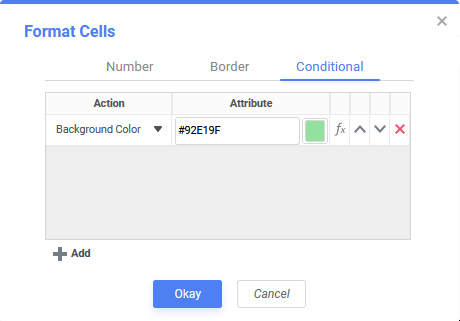
Conditional format tab of Format Cells dialog
- Click
 Add to create a new condition.
 - From the Action list, select an action to occur if the condition is met. If applicable, select an attribute for the action from the Attribute list.
Action Attribute Foreground Color Enter a formula, hexadecimal color code or select a color using the color picker which will change the foreground (text) color of the chosen cell. Background Color Enter a formula, hexadecimal color code or select a color using the color picker which will change the background color of the chosen cell. Font Family Select a font to change the text to. Font Size Enter a font size, in ems, to change the font size to. Bold no attribute Italic no attribute Underline no attribute Horizontal Alignment Choose from Left, Right, Center or Justify to which the text in the cell will change to. Vertical Alignment Choose from Top, Middle or Bottom to which the text in the cell will change. Suppress Row no attribute Suppress Section no attribute Page Break no attribute Tip
Hexadecimal color values may be upper or lowercase and may contain the # prefix character, but it is not required.
- Click the Formula Editor icon to enter a formula for the condition. The formula must evaluate to True or False. The Action will be applied to the report when the formula evaluates to True.
To use the value of the current cell in the formula, use the function
CellValue(). Click Cell Value to insert CellValue()into the formula.
 Add to create a new condition.
A cell can have multiple conditional formats, each of which is a separate row in the Conditional tab. If two or more overlap, the lower condition takes precedence. Click the Move Row Up and Move Row Down
 icons to reorder the precedence of the conditions.
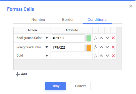
Multiple conditions and formats may be added for a cell
Using Formulas as Conditional Formatting Colors v2019.2+
In addition to selecting a static color with the color selector, a formula may be used to change the colors of a cell when conditional formatting.
A formula which returns a value convertible to a hexadecimal color code can be entered as the Attribute when the Action is Foreground Color or Background Color. When using this option, conditional formatting color properties can be determined at runtime instead of report design time.
One application of this feature is to read color values from a data source and use that color data to apply formatting to a cell.
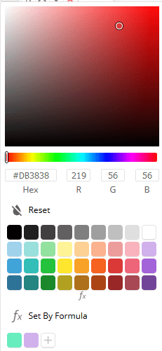
Clicking on the Color Selector‘s  Set by Formula button will open the standard Formula Editor. All formula elements available in conditional formulas are available, including
 CellValue(), references to other cells, application parameters and Data Objects. Aggregate functions are not available in attribute formulas.
Tip
Hexadecimal color values may be upper or lowercase and may contain the # prefix character, but it is not required.
If the formula returns null or an empty string, the conditional formatting is not applied. If the formula returns a value that is not convertible to a hexadecimal color code, an error message is displayed in the cell.
Examples
This example uses conditional and logical functions to combine multiple conditions into one clause.
If(And(CellValue()>=1000, CellValue()<10000), "#FFFFFF", If(CellValue()>=10000, "#ECECEC", "#00000"))
This example uses an application parameter named ConditionalColor to select a color to apply:
=@ConditionalColor@
This example simply refers to a Data Field that contains a hexadecimal color value to apply:
{Products.ProductColor}
A few examples of valid hexadecimal color codes:
#FFF
#c0c0c0
ff4c00
F90